Basics

Rotation matrix¶

\(R\cdot R^T = I\) --> \(R^{-1} = R^T\)
det(R) = +1 --> Right System resultierende Abbildung ist Rotation
det(R) = -1 --> Left System resultierende Abbildung ist Spiegelung
use the right hand rule!

\[ \mathbf{R}_x = \begin{bmatrix}1 & 0 &0 \\ 0 & cos(\alpha) & -sin(\alpha) \\ 0 & sin(\alpha) & cos(\alpha)\end{bmatrix}, \quad \mathbf{R}_y = \begin{bmatrix}cos(\beta) & 0 &sin(\beta) \\ 0 & 1 & 0 \\ -sin(\beta) & 0 & cos(\beta)\end{bmatrix} \]

\[ \mathbf{R}_z = \begin{bmatrix}cos(\gamma) & -sin(\gamma) &0 \\ sin(\gamma) & cos(\gamma) & 0 \\ 0 & 0 & 1\end{bmatrix} \]

Example

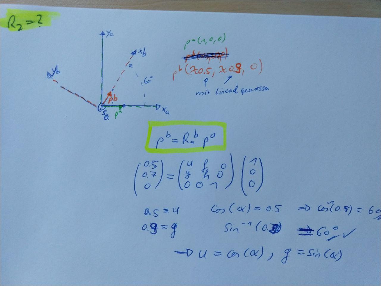
Rotation of a coordinate frame

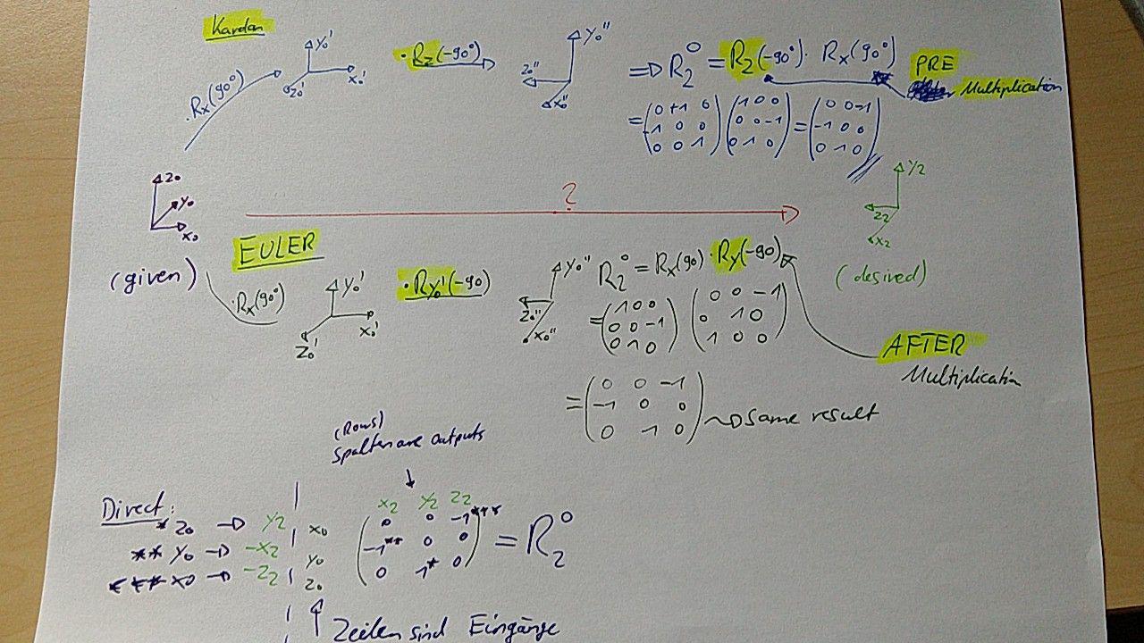
There are two types of chained rotations

pre-multiplication (kardan angle), new rotation matrix is multiplied to the left side:
- The reference frame is always the same:
- \(R^a_b = R_{new} \cdot R_1\)
- Frame \(S_b\) will be rotated around the fixed axis of \(S_a\)
after-multiplication (euler angle), new rotation matrix is multiplied to the right side
- The reference is the current frame \(S_b\)
- \(R^a_b = R_1 \cdot R_{new}\)
- Relative rotation, according to the current frame.

Kardan angle (RPY -angle)

ZYX: \(\phi\), roll (around Z-axis), \(\theta\) pitch (around y axis) and \(\psi\) yaw (around x axis)
Premultiplication is used:
\(R_b^a(\psi, \theta, \phi) = R_z \cdot R_y \cdot R_x\)=

\[ \begin{bmatrix}cos(\phi) & -sin(\phi) &0 \\ sin(\phi) & cos(\phi) & 0 \\ 0 & 0 & 1\end{bmatrix} \cdot \begin{bmatrix}cos(\theta) & 0 &sin(\theta) \\ 0 & 1 & 0 \\ -sin(\theta) & 0 & cos(\theta)\end{bmatrix} \cdot \begin{bmatrix}1 & 0 &0 \\ 0 & cos(\psi) & -sin(\psi) \\ 0 & sin(\psi) & cos(\psi)\end{bmatrix} \]

\[ = \left( \begin{array}{ccc}{\cos \phi \cos \theta} & {-\sin \phi \cos \psi+\cos \phi \sin \theta \sin \psi} & {\sin \phi \sin \psi+\cos \phi \sin \theta \cos \psi} \\ {\sin \phi \cos \theta} & {\cos \phi \cos \psi+\sin \phi \sin \theta \sin \psi} & {-\cos \phi \sin \psi+\sin \phi \sin \theta \cos \psi} \\ {-\sin \theta} & {\cos \theta \sin \psi} & {\cos \theta \cos \psi}\end{array}\right) \]

If you have a Rotation matrix and want to obtain \(\theta, \psi, \phi\) then do:

\(R_{3,1} = -sin(\theta)\) --> \(\theta\)
\(R_{3,2} = cos(\theta) sin(\psi)\) --> \(\psi\) use \(R_{3,3}\) to test it.
\(R_{1,1} = cos(\phi)cos(\theta)\) --> \(\phi\)

Euler angle (ZYZ -angle)

use chained rotation's of the current reference system
After multiplication: R_b^a = R_z \cdot R_y \cdot R_z
or Bryant-angle (ZYX) are also common.

Example: Kardan vs. Euler

kardan_vs_euler

Quaternions

as Euler or Kardan has not always a unique solution use quaternions
Quaternion \(\mathbf{q} = \begin{bmatrix} x & y & z & w \end{bmatrix}^T\)
\(\mathbf{q} = w+xi+yj+zk\), \quad \(i^2=j^2=k^2 = -1, \quad ij=k=-ji, \quad x,y,z,w \in \mathbb{R}\)

Rules of Quaternions:

\[ \mathbf{q_1} = \begin{bmatrix}\mathbf{a}_1\\w \end{bmatrix}, \quad \mathbf{q_2} = \begin{bmatrix}\mathbf{a}_2\\w \end{bmatrix}, \quad \mathbf{a}_1 = \begin{bmatrix} x \\ y \\ z \end{bmatrix} \]

\(\mathbf{\vert{q}\vert} = 1\) (normalized quaternion)
\(\mathbf{q}_1 + \mathbf{q}_2 =\begin{bmatrix} \mathbf{a}_1+\mathbf{a}_2 & w_1 + w_2 \end{bmatrix}^T\)
\(\b{q}_1 \cdot \mathbf{q}_2 = \begin{bmatrix} w_1 w_2 - \mathbf{a}_1^T \mathbf{a}_2 & \mathbf{a}_1 \times \mathbf{a}_2 + w_1 \mathbf{a}_2 + w_2 \mathbf{a}_1 \end{bmatrix}^T\)
\(\b{q}^{-1} = \frac{1}{w^2+x^2+y^2+z^2} \cdot [-\b{a}, w]^T\)
From quaternion to rotation matrix:

\[ R=\left( \begin{array}{ccc}{1-2\left(y^{2}+z^{2}\right)} & {2(x y-z w)} & {2(x z+y w)} \\ {2(x y+z w)} & {1-2\left(x^{2}+z^{2}\right)} & {2(y z-x w)} \\ {2(x z-y w)} & {2(y z+x w)} & {1-2\left(x^{2}+y^{2}\right)}\end{array}\right) \]

Transformation¶

If you want to express a position vector \(\mathbf{p^b}\) in another coordinate system \(S_a\) you need the Rotation matrix \(\mathbf{R_b^a}\) (from coordinate System \(S^a\) to \(S_b\)) and the translation vector \(\mathbf{r^a_b}\) (distance vector between the two coordinate systems)

Position

\[ \mathbf{p}^a = \mathbf{r}^a_b + \mathbf{R}^a_b \mathbf{p}^b \\ \mathbf{p}^0(t) = \mathbf{r}^0_n(\b{q}(t)) + \mathbf{R}^0_n(\b{q}(t)) \mathbf{p}^n(t) \]

Velocity

\[ \b{p}^0(t) = \dot{\b{r}^0_n(\b{q}(t))} + \dot{\b{R}^0_n(\b{q}(t))} \b{p}^n(t)+ {\b{R}^0_n(\b{q}(t))} \dot{\b{p}^n(t)} \]

Acceleration

contains linear, coriolis and zentrifugal part.

Homogeneous Transformation¶

\[ \begin{bmatrix} \mathbf{p^a} \\ 1 \end{bmatrix} = \underbrace{\begin{bmatrix} R_b^a & r_b^a \\ \mathbf{0}^T & 1 \end{bmatrix}}_{T_b^a} \cdot \begin{bmatrix} \mathbf{p^b} \\ 1 \end{bmatrix} \]

inverse homogeneous transformation

\[ {T_b^a}^{-1} = T_a^b = \begin{bmatrix} {R_b^a}^T &-{R_b^a}^T \cdot r_b^a \\ \mathbf{0}^T & 1 \end{bmatrix} \]

Kinematics (position)¶

Assume a robot (arm) consists of revolute joints (\(\theta_i\)) and prismatic joints (\(d_i\)). The goal is to find the joint angles(\(q_i\)) for a desired pose (position + orientation) of the endeffector (tip position of the robot arm). This is called Inverse Kinematics. If you want to calculate the tip position of the robot arm with given joint angles is named Direct Kinematics:

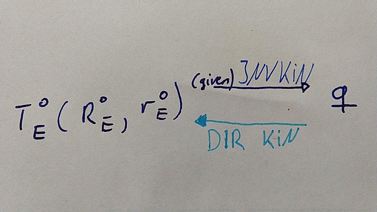
First DIR-KIN is discussed. This can be done using Denavit Hartenberg.

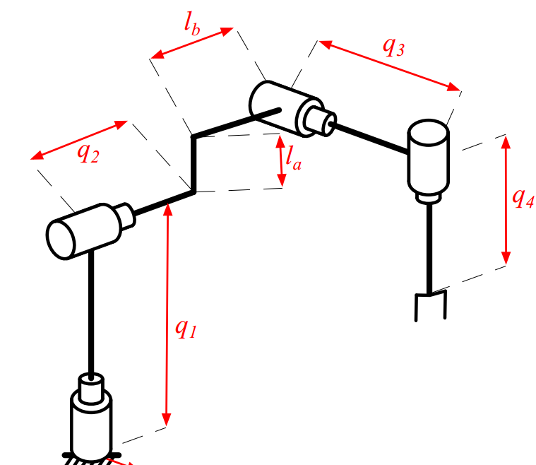
Denavit Hartenberg - Direct Kinematics¶

Video example

(Assumption): Nullposition arms, etc. are streched out
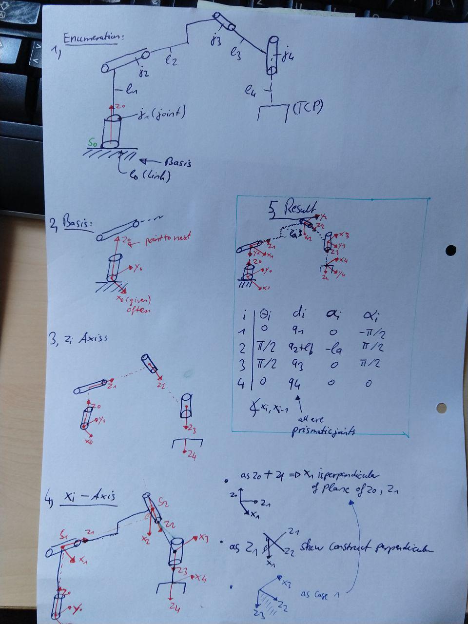
Enumeration of all Joints (j) and Links (l) and Frame System (S)

--> Basis: \(S_0\) origin on \(z_0\). \(x_0, y_0\) as right system
Declaration of the \(z_i\) axis:

--> prismatic joint \(z_0\) points to next joint (i+1)

--> revolute joint \(z_0\) rotates with respect to right hand rule and points to next joint (i+1)
The origin of \(S_i\) is set to:

--> If \(z_{i-1}, z_i\) cross: Intersection point = origin of \(S_i\)

--> If \(z_{i-1}, z_i\) are parallel: Origin \(S_i\) is on \(z_i\) on the joint \(z_{i+1}\)

--> If \(z_{i-1}, z_i\) are skew-wiff: Construct common perpendicular, intersection point on \(z_i\) is origin of \(S_i\)
The \(x_i\) axis is set to:

--> If \(z_{i-1}, z_i\) cross: \(x_i\) axis points to the perpendicular of the plane which is created by \(z_i\) and \(z_{i-1}\)

--> If \(z_{i-1}, z_i\) are parallel: \(x_i\) axis points to the next joint (i+1) along the perpendicular of \(z_i\) and z_\(i-1\) through \(S_i\)

--> If \(z_{i-1}, z_i\) are skew-wiff: \(x_i\) axis points in the direction of the perpendicular through \(S_i\) such that \(x_i\) intersects \(z_{i-1}\)
The \(y_i\) axis are set such that a right system is created
The Endefector coordinate frame \(S_n\) is set to the Tool Center Point

--> Set \(S_n\) such that DH Table contains as much zeros as possible

Construct DH-Table:

Joint \(i\)	\(\theta_i\)	\(d_i\)	\(a_i\)	\(\alpha_i\)
1,....n	angle between \(x_{i-1}\) and \(x_i\) measured around \(z_{i-1}\)	Distance between \(S_{i-1}\) along \(z_{i-1}\) to intersection with \(x_i\)	Distance between intersection \(z_{i-1}\) and \(x_i\) axis to \(S_i\) along \(x_i\) axis	angle between \(z_{i-1}\) and \(z_i\) measured around \(x_i\) if \(z_1 \vert \vert z_2 \rightarrow = 0\)

Calculate the Transformation matrix from the basis frame to the endefector using the DH Table

\[ T_i^{i-1} = R_{z,i}(\theta_i) \cdot Trans(0,0,d_i) \cdot Trans(a_i,0,0) \cdot R_{x,i}(\alpha_i) \\ T_n^0 = T_1^0 \cdot T_2^1 \cdot \cdot \cdot T_n^{n-1} \]

Pyhton code to calculate T from 0 to endeffector

#DH tabel converter
import numpy as np
from math import pi
from sympy import *
from sympy import pprint

#numpy arrays 
def R_matrix(i,symbol):
    #i=1: x rotation matrix
    #symbol="q1" or value
    #print(type(symbol))

    if isinstance(symbol, str):
    x=Symbol(symbol)
    else:
    x=symbol

    R= eye(3)#work with sympy
    if i==1:
    R[1,1]=cos(x)
    R[1,2]=-sin(x)
    R[2,1]=sin(x)
    R[2,2]=cos(x)

    if i==3:
    R[0,0]=cos(x)
    R[0,1]=-sin(x)
    R[1,0]=sin(x)
    R[1,1]=cos(x)
    return R

def T_matrix(R_matrix,r_vector):
    T= Matrix([[0,0,0,1]])
    R_matrix=R_matrix.col_insert(3,Matrix([[0],[0],[0]]))
    T=T.row_insert(0,R_matrix[0,:])
    T=T.row_insert(1,R_matrix[1,:])
    T=T.row_insert(2,R_matrix[2,:])
    r_vector = r_vector.row_insert(3, Matrix([[0]]))
    T[:,3]= r_vector
    T=T.row_insert(3,Matrix([[0,0,0,1]]))
    T.row_del(4)
    return T

def calculate_dh(theta,d,a,alpha):
    res = []
    for i in range(0,len(theta)):
    tmpz=T_matrix(R_matrix(3,theta[i]),(Matrix([[0],[0],[d[i]]])))
    tmpx=T_matrix(R_matrix(1,alpha[i]),(Matrix([[0],[0],[a[i]]])))
    res.append(tmpz*tmpx)
    return res

def calculate0TE(res):
    if len(res)>1:
    tmp1 = res[0]
    tmp2 = res[1]
    del res[1]
    res[0]=tmp1*tmp2
    return simplify(calculate0TE(res))
    else:
    return res[0]
#T_matrix(R_matrix(1,"a"),Matrix([["q1"],[2],[15]]))
res=calculate_dh([0,"q1+pi/2",0,"q3",0],["l1",0,"q2",0,"q4"],[0,0,0,0,0],[0,pi/2,-pi/2,pi/2,0])
pprint((calculate0TE(res)))

Example DH

Inverse Kinematics¶

Find the solution of \(3\cdot3 +3 = 12\) non-linear equations that map from \(T_0^E\) to \(\b{q}\).
Assuming that \(R_0^E\) is expressed in 3 Euler or Kardan angles there are only 6 non-linear equations
We want to find a \(\b{q}\) such that: \(T_0^E(\b{q}) = \tilde{T}_{E, given}\), the 6 non-linear equations are:
- \(r_{E,1}^0(\mathbf{q}) - \tilde{r}_{E,1}^0 = 0\)
- \(r_{E,2}^0(\mathbf{q}) - \tilde{r}_{E,2}^0 = 0\)
- \(r_{E,3}^0(\mathbf{q}) - \tilde{r}_{E,3}^0 = 0\)
- \(\alpha(\b{q}) - \tilde{\alpha}=0\)
- \(\beta(\b{q}) -\tilde{\beta}=0\)
- \(\gamma(\b{q})- \tilde{\gamma}=0\)
Solving these 6 equations depends on the number of joints q:
- if \(q<6\) no solution
- if \(q=6\) exaclty one solution --> This is the reason many robots have 6 joints (6DoF)
- if \(q>6\) redundancy multiple solutions (ellbow high, low)

Solving INV-KIN

analytical (geometrical or algebraric works by hand for 2-DoF)
numerical (iterative) works for higher DoF

Libraries in use: openrave -> ikfast, kdl, Drake (iterative)

For my local ROS-Kuka-Arm project I used from trac_ik_python.trac_ik import IK

Jacobian (velocity)¶

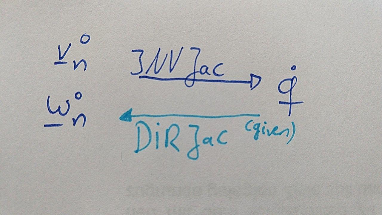
There are basically 2 ways to calculate the Jacobian Matrix.

Get the Jacobian with the \(T_{i-1}^0\) using DIR-KIN
- If \(q_i = \theta_i\) (revolute joint)
  - \(J_{n,i}^0 = \begin{bmatrix}e_{z,i-1}^0 \times (r_n^0- r_{i-1}^0) \\ e_{z,i-1}^0 \end{bmatrix}\)
- If \(q_i = d_i\) (prismatic joint)
  - \(J_{n,i}^0 = \begin{bmatrix} e_{z,i-1} \\ \b{0} \end{bmatrix}\)
- This solution is derived by derivating \(\mathbf{p}^a = \mathbf{r}^a_b + \mathbf{R}^a_b \mathbf{p}^b\) to the time
Get Jacobian with just T_n^0
- \(v_n^0 (t) = \dot{r}_n^0(\b{q}(t)) = \frac{\partial r_n^0(\b{q}(t)}{\partial \b{q}} \cdot \dot{\b{q}}(t)\)
- \(\omega_n^0(t): B(q(t), \dot{q}(t))= \frac{\partial R(q(t))}{\partial q(t)} \cdot \dot{q}(t) \cdot R^T(q(t))\)
  - get \(\omega_x, \omega_y, \omega_z\) by comparing the matrix with B see below
- This solution can be derived by derivating \(R(\b{q}(t)) \cdot R^T(\b{q}(t))\) to the time.

with:

\[ T_i^0(\b{q}) = \begin{bmatrix} e_{x,i}^0 & e_{y,i}^0 & e_{z,i}^0 & r_i^0 \\ 0 & 0 &0 &1 \end{bmatrix} \\ B = \begin{bmatrix} 0& -\omega_z & \omega_y \\ \omega_z & 0 &-\omega_x\\ - \omega_y & \omega_x & 0 \end{bmatrix} \]

(example!)

Dynamics (torques, forces)¶

Direct Dynamics (DIR-DYN)¶

Inverse Dynamics (INV-DYN)¶

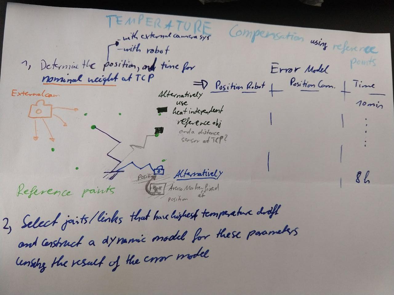
Temperature Compensation of Industrial Robots (IR)¶

Industrial Robots require a high positioning accuracy
A time independent repeatability as well as an absolute accuracy (Pose Genauigkeit nach DIN-ISO 9283) is desired
It is not possible to prevent all internal and external heat sources --> temperature drift occurs
A calibration system is desired to achieve a high precision (repeatability and absolute acc.) is desired

Approaches¶

use thermometer's to measure the temperature and correct the TCP position with the measured values -> expensive (many thermometers's) in total measuring the temperature is an inefficient way that does not directly correlate to the error of the TCP.
Develop a gauging (eichungs) system ?
3D-Messsystem RX-Frams by Stäubli developed 2006?
Dynaloag AutoCal Series 2 System uses twin beam lasers and reference points
Compensation of Errors in Robot Machining (Bearbeitungsroboter) With a Parallel 3D-Piezo Compensation Mechanism: error smaller than 0.0335 mm
Temperaturverformungsmodelle: Erfassung und Ausgleich thermisch bedingter Verformungen an Industrierobotern. Tübingen: MVK Medienverlag Köhler, 1998

3D-Piezo-Ausgleichsaktorik, Diss, 2011, Stutt

Temperaturmodelle ermöglichen die Kompensation durch bekannte reversibel und reproduzierbar stattfindende Erwärmungszustände des Robotersystems. Hierbei stehen die Kompensationsdaten als Korrekturwerte in allen relevanten Posen bei den jeweiligen Betriebszuständen zur Verfügung. Dies hat den Nachteil, dass Umgebungszustände exakt definiert und Änderungen des Programms in allen Betriebsbedingungen berücksichtigt werden müssen. Temperaturverformungsmodelle berücksichtigen offline Simulation nach der Finite Elemente Methode (FEM) der jeweiligen Verformungszustände des Roboters. Diese werden sensorisch mit Hilfe an der Roboterstruktur aufgebrachten Sensoren ermittelt.
using reference points:

Links¶

Industrial Robots¶

Properties¶

Pose repeatability e.g. \(\pm 0.04 mm\)
Number of axis e.g. 6
Volume of working envelope (Arbeitsraum) e.g. 8.4 m³
Payload (Nutzlast)
absolute accuracy e.g. \(\leq 1 mm\)

General aspects¶

closed kinematic chains are stiffer
precision is divided in pose and trajectory (repeatability and absolute)
Compensation is done during the process
Calibration is done before starting the process (during the startup (Inbetriebnahme))
- an efficient method is the model based calibration

Robotics dictionary¶

Englisch	Deutsch
revolute joint	Drehgelenk
prismatic joint	Schiebungsgelenk
(rigid) link	(starrer) Glied
joint	Gelenk
task space	given x(t) endeffector traj.
joint space	required: controls u, given q,qdot,qdotdot