Basics

Basic Maths

There are nice explanation videos of the below topics by 3blue1brown.

Eigenvalues

To calculate the Eigenvalues of Matrix A:

\[ det(sI-A)=0 \]

Example: (To-Do)

To approximate Eigenvalues use Gershgorin.

Eigenvectors

To calculate the Eigenvectors of the Eigenvalues \(s_i\):

\[ (s_i I-A)v_i=0 \]

Determinant

If the rank( A ) = 0 --> det(A) = 0, then the inverse of A cannot be calculated.

For 2x2 Matrix:

\[ det(\begin{bmatrix} a&b\\c&d \end{bmatrix}) = a d - c b \]

For 3x3 Matrix: The fastest way is to do it by coloums or by rows and use the chessboard pattern for the sign of the subdeterminants.

Do it for first column:

\[ det(\begin{bmatrix} a&b&c\\d&e&f\\g&h&i \end{bmatrix} = + det(\begin{bmatrix} e&f\\ h&i \end{bmatrix}) - det(\begin{bmatrix} b&c\\ h&i \end{bmatrix})+ det(\begin{bmatrix} b&c\\ e&f \end{bmatrix}) \]

The 2x2 subdeterminants are calculated as described above.

The sign of the subdeterminants is given by:

\[ det(\begin{bmatrix} +&-&+\\-&+&-\\+&-&+ \end{bmatrix} \]

Example for a 4x4 Matrix:

Example from Engine:

If you want to calculate the Determinant of a symbolic or numerical Matrix online simply copy the Code below in the input area of simact Engine and click RUN.

A = [[1,2],[3,4]]
det(A)

Inverse

The inverse can only be calculated for square matrices. If rank(A) = 0 --> det(A) = 0 --> inverse of A cannot be calculated.

For a 1x1 Matrix:

\[ inv(a) = 1/a \]

For a 2x2 Matrix:

\[ inv(\begin{bmatrix} a&b\\c&d \end{bmatrix} = \frac{1}{der(\begin{bmatrix} a&b\\c&d \end{bmatrix})} \cdot \begin{bmatrix} d&-b\\-c&a\end{bmatrix} \]

For a 3x3 Matrix:

\[ inv(\begin{bmatrix} a&b&c\\ d&e&f \\ g&h&i \end{bmatrix} =\frac{1}{ det(\begin{bmatrix} a&b&c\\ d&e&f \\ g&h&i \end{bmatrix}) } \cdot \begin{bmatrix} +det(\begin{bmatrix}e&f\\h&i\end{bmatrix} ) a&b&c\\ d&e&f \\ g&h&i \end{bmatrix} \]

For a 4x4 Matrix: For this big Matrix use either the Engine or find the Matrix that is mulitiplicated with original to get the Identity Matrix:

\[ \mathbf{A} \mathbf{B} = \mathbf{I} \]

Then

\[ \mathbf{ B}= inv(\mathbf{A}) \]

For diagonal matrices:

Frequenzkennlinienverfahren

Ortskurven (Nyquist)

Root locus method Wurzelortskurvenverfahren

This method can be used to see how eigenvalues of a system change if one parameter e.g. the gain of a transfer function is changing. Thereby the desired K can be found to stabilize a system. Assume the following control circuit:

The open loop transfer function is giving by:

\[ G_o = G_r(s) G_s(s) = k \frac{Z_o(s)}{N_o(s)} \]

\(Z_o\) is the nominator and \(N_o\) the denominator. The closed loop transfer function of the above control circuit is:

\[ G_c(s) = \frac{G_o}{1+G_o \cdot G_m } = \frac{k Z_o}{N_o + k Z_o} \text{ If } Gm = 1 \]

Then the characteristic equation that is used for the root locus method is the denominator of the above equation:

\[ \underbrace{N_o}_{P_2} + k \underbrace{Z_o}_{P_1} = 0 \rightarrow k = - \frac{N_o}{Z_o} \]

These are basically two polynoms. The Polynom that is multiplied by \(k\) should have higher or equal order: \(P_2 >= P_1\)

With the open loop transfer function the algebraic equation can be construed:

\[ RE(Z_o) IM(N_o) - IM(Z_o) RE(N_o)=0 \]

using \(s= \sigma + j \omega\) one can draw the root locus for the algebraic equation if \(grad(N_o)+grad(Z_o)<=6\). Note that there is no k in the above equation.

The algebraic equation can be often formulated as Hyperbole:

\[ \frac{(x - x_0)^2}{a^2} - \frac{(y-y_0)^2}{b^2}= 1 \]

or as ellipse:

\[ \frac{(x - x_0)^2}{a^2} + \frac{(y-y_0)^2}{b^2} = r^2 \]

Example draw root locus of algebraic equation:

Todo: Code this for the engine

Rules of root locus:

The root locus is a continuous line that connects the poles to the zeros (or goes to bed infinity) of the open loop transfer function \(G_o(s)\) for k>0. In general it can be said that zeros attract branches of the root locus. Poles repel branches of the root locus.

• Draw the n Poles(×) and m Zeros (o).
• The root locus (rl) is symmetrical to the real axis. The real axis always belongs to the rl either for k>0 or k<0.
• If a pole is double (or of n order) then two (n) branches of the rl go out of this pole.
• Draw the rl on the real axis: If the number of poles and zeros right of a current pole is uneven then it belongs to the rl for k>0. Otherwise to k<0.
• To calculate the intersection points (\(s_i\)) of branches of the rl:

\[ \frac{1}{s-n_1}+...+\frac{1}{s-n_n} - [\frac{1}{s-p_1}+\frac{1}{s-p_n}] = 0 \]

• Intersection angle in the intersection point:

\[ \Phi = \frac{\pi}{\text{number of branches in intersection point}} \]

• Calculation of the asymptote intersection point also known as root Schwerpunkt:

\[ \sigma_s = \frac{Re(n_1+...+n_n)-Re(p_1+...+p_n)}{m-n} \]

• Inclination angle of asymptote. There are i angles of a asymptote intersection point.

for k>0:

\[ \varphi_i = \frac{(2 i +1) \pi}{n-m} \]

for k<0:

\[ \varphi_i = \frac{(2 i) \pi}{n-m} \]

• Intersection point of rl with IM axis(\(s=j\omega\)):

\[ IM(N_o(s)+kZ_o(s)) = 0 \rightarrow k = ... \]

\[ RE[N_o(s)+kZ_o(s)] = 0 \rightarrow \omega=... \]

Analytical solution of differential equations in time domain (Anfangswertproblem)

To solve linear differential equations of \(n^{th}\) order that look like:

\[ a_n y^{(n)}(t) + . . . + a_2 \ddot{y}(t) + a_1 \dot{y}(t) + a_0 y(t) = r(t) \]

The general solution is:

\[ y(t) = y_{homogen} + y_{particular} \]

For the homogeneous solution the right side \(r(t) =0\):

Approach:

\[ y(t) = e^{\lambda t} \rightarrow \dot{y}(t) = \lambda e^{\lambda t}, ... \]

Insert it in Differential Equation and divide through \(e^{\lambda t}\) gives the characteristic Polynom \(P(\lambda)\). Then calculate the zeros \(\lambda_i\) of this Polynom and insert them in the approach. This gives:

\[ y(t) = \sum_{i=1}^n c_i e^{\lambda_i t} \]

\(c_i\) can be calculated by using the initial values. This equation holds for single real Eigenvalues. If Eigenvalues are double use:

\[ y(t) = c_1 e^{\lambda_1 t}+ c_2 t e^{\lambda_1 t} \]

To solve the particular equation:

Example of a mass spring damper system:

The differential equation of a single mass spring damper system is given by:

\[ m \ddot{x}(t) + k x(t) + b \dot{x} (t) = F(t) \]

First solve the homogeneous equation for \(F(t)=0\). Inserting the above approach gives the characteristic Polynom \(P(\lambda)\):

\[ \lambda^2 m + \lambda b + k = 0 \rightarrow \lambda_{1,2} = \frac{-b \pm \sqrt{b^2 - 4\cdot m k}}{2m} \]

Let's assume \(m=2\) kg \(b=4\), k= \(2\):

\[ \lambda_{1} = -0.5 \quad \lambda_2 = -1.5 \rightarrow y_h(t) = x(t) = c_1 e^{\lambda_1 t} + c_2 e^{\lambda_2} \]

Now assume the initial position and velocity of the mass to be zero:

\[ x(t=0) = 0, \quad \dot{x}(t=0) = 0 \\ \rightarrow c_1 =- c_2, \\ \rightarrow -c_2 \lambda_1 + c_2 \lambda_2 = 0 \\ c_2 = \lambda_2-\lambda_1 \]

The homogeneous solution is:

\[ x(t) =e^{-0.5 t} - e^{-1.5 t} \]

Solve a System of a second order differential equations

See also here.

Assume you have the following differential equation system:

\[ \mathbf{M} \ddot{\mathbf{x}} + \mathbf{C} {\mathbf{x}} = 0 \\ \mathbf{M} = \begin{bmatrix} m_1 & 0 & 0 &0 &0 &0 \\ 0 & m_2 & 0 &0 &0 &0 \\ 0 & 0 & m_3 &0 &0 &0 \\ 0 & 0 & 0 &m_4 &0 &0 \\ 0 & 0 & 0 &0 &0 &m_5 \\ \end{bmatrix} \\ \mathbf{C} = \begin{bmatrix} c_1+c_5 & -c_1 & 0 &0 &-c_5 \\ -c_1& c_1+c_2+c_3&-c_2&-c_3&0\\ 0&-c_2&c_2&0&0 \\ 0&-c_3&0&c_3+c_4&-c_4\\ -c_5&0&0&-c_4&c_4+c_5 \\ \end{bmatrix} \]

This is a homogenous second order differential equation system which corresponds to a mass(m1-m5) spring(c1-c5) system.

To calculate the eigenvalues first transform it to a first order differential equation system using \(\mathbf{v}(t) = \dot{\mathbf{x}}(t)\):

\[ \mathbf{M} \ddot{\mathbf{x}} + \mathbf{C} {\mathbf{x}} = 0 \\ \rightarrow \ddot{\mathbf{x}}(t) = \dot{\mathbf{v}}(t) = -\mathbf{M}^{-1} \cdot \mathbf{C} \mathbf{x} (t) \]

Next construct a system of differential equations which contains first oder and second oder differential equations:

\[ \begin{bmatrix} \mathbf{v} = \mathbf{\dot{x}} \\ \mathbf{\dot{v}} = \mathbf{\ddot{x}} \end{bmatrix} = \begin{bmatrix} \mathbf{0} & \mathbf{I} \\ \mathbf{A} & \mathbf{0} \end{bmatrix} \cdot \begin{bmatrix} \mathbf{x} \\ \mathbf{\dot{x}} \end{bmatrix} \\ \mathbf{A} = \mathbf{M}^{-1} \cdot \mathbf{C} \]

Next calculate the \(n\) Eigenvalues \(\lambda_i\) of this System:

\[ det(s\mathbf{I} - \mathbf{B}) = 0, \quad \mathbf{B} = \begin{bmatrix} \mathbf{0} & \mathbf{I} \\ \mathbf{A} & \mathbf{0} \end{bmatrix} \]

Then calculate the \(n\) Eigenvectors \(v_i\) to these \(\lambda_i\) (e.g. with Matlab).

If all Eigenvalues of B are now single (no double Eigenvalues) then the time solution for the velocity (how the velocity of the masses oscillates) is given by:

\[ \mathbf{\hat{x}}(t) = \sum_{i=1}^{n} e^{\lambda_i} t \cdot v_i \cdot c_{i,0} \\ \mathbf{\hat{x}}(t) = \begin{bmatrix} \mathbf{x} \\ \mathbf{\dot{x}} \end{bmatrix} \]

\(c_{i,0}\) are constants. These constants can simply be found out with the initial values:

\[ \mathbf{\hat{x}}(t=0) = \begin{bmatrix} \mathbf{x}_0 \\ \mathbf{v}_0 \end{bmatrix} \]

\(\mathbf{\hat{x}}\) is a 10x1 vector for the above 5x5 second order diff. eq. system that stores the velocity and positioning solution.

Matlab script

clear; clc;
m1 = 3;
m2 = 4;
m3 = 5;
m4 = 6;
m5 = 7;
c1 = 21;
c2 = 2;
c3 = 31;
c4 = 4;
c5 = 51;

x0 = [1 ; 0 ; 0 ; 0 ; 0];
v0 = [-10 ; 0 ; 0 ; 0 ; 0];

M = diag([m1,m2,m3,m4,m5]);
C = [c1+c5,-c1,0,0,-c5;
    -c1, c1+c2+c3,-c2,-c3,0;
    0,-c2,c2,0,0;
    0,-c3,0,c3+c4,-c4;
    -c5,0,0,-c4,c4+c5];

A = -inv(M)*C;
B = [zeros(5,5), eye(5); A, zeros(5,5)]
[eigvectors, eigvalues] = eig(B)
lambda = diag(eigvalues)

syms t v1 v2 v3 v4 v5 v6 v7 v8 v9 v10
v = exp(lambda(1)*t)*eigvectors(:,1)*v1+...
    exp(lambda(2)*t)*eigvectors(:,2)*v2+...
    exp(lambda(3)*t)*eigvectors(:,3)*v3+...
    exp(lambda(4)*t)*eigvectors(:,4)*v4+...
    exp(lambda(5)*t)*eigvectors(:,5)*v5+...
    exp(lambda(6)*t)*eigvectors(:,6)*v6+...
    exp(lambda(7)*t)*eigvectors(:,7)*v7+...
    exp(lambda(8)*t)*eigvectors(:,8)*v8+...
    exp(lambda(9)*t)*eigvectors(:,9)*v9+...
    exp(lambda(10)*t)*eigvectors(:,10)*v10;

vv = subs(v,t,0);
L = solve(vv == [x0; v0] , v1, v2, v3, v4, v5, v6, v7, v8, v9, v10);

v1w = L.v1;
v2w = L.v2;
v3w = L.v3;
v4w = L.v4;
v5w = L.v5;
v6w = L.v6;
v7w = L.v7;
v8w = L.v8;
v9w = L.v9;
v10w = L.v10;

v = subs(v, [v1, v2, v3, v4, v5, v6, v7, v8, v9, v10], [v1w, v2w, v3w, v4w, v5w, v6w, v7w, v8w, v9w, v10w]);
x_hat = vpa(v,2) %round it

%     exp(t*(2.2e-16 - 9.9e-9i))*(0.06 - 6.1e7i) + exp(t*(2.2e-16 + 9.9e-9i))*(0.06 + 6.1e7i) + exp(t*(1.7e-16 - 2.0i))*(0.035 - 0.18i) + exp(t*(1.7e-16 + 2.0i))*(0.035 + 0.18i) + exp(t*(7.2e-17 - 5.6i))*(0.36 - 0.65i) + exp(t*(7.2e-17 + 5.6i))*(0.36 + 0.65i) + exp(t*(- 4.4e-17 - 0.7i))*(0.017 - 0.24i) + exp(t*(- 4.4e-17 + 0.7i))*(0.017 + 0.24i) + exp(t*(3.0e-17 - 4.0i))*(0.024 - 0.061i) + exp(t*(3.0e-17 + 4.0i))*(0.024 + 0.061i)
%                    exp(t*(2.2e-16 - 9.9e-9i))*(0.06 - 6.1e7i) + exp(t*(2.2e-16 + 9.9e-9i))*(0.06 + 6.1e7i) - exp(t*(1.7e-16 - 2.0i))*(0.032 - 0.16i) - exp(t*(1.7e-16 + 2.0i))*(0.032 + 0.16i) - exp(t*(7.2e-17 - 5.6i))*(0.12 - 0.21i) - exp(t*(7.2e-17 + 5.6i))*(0.12 + 0.21i) + exp(t*(- 4.4e-17 - 0.7i))*(0.013 - 0.19i) + exp(t*(- 4.4e-17 + 0.7i))*(0.013 + 0.19i) + exp(t*(3.0e-17 - 4.0i))*(0.076 - 0.19i) + exp(t*(3.0e-17 + 4.0i))*(0.076 + 0.19i)
%  exp(t*(2.2e-16 - 9.9e-9i))*(0.06 - 6.1e7i) + exp(t*(2.2e-16 + 9.9e-9i))*(0.06 + 6.1e7i) + exp(t*(1.7e-16 - 2.0i))*(3.7e-3 - 0.019i) + exp(t*(1.7e-16 + 2.0i))*(3.7e-3 + 0.019i) + exp(t*(7.2e-17 - 5.6i))*(1.5e-3 - 2.7e-3i) + exp(t*(7.2e-17 + 5.6i))*(1.5e-3 + 2.7e-3i) - exp(t*(- 4.4e-17 - 0.7i))*(0.063 - 0.91i) - exp(t*(- 4.4e-17 + 0.7i))*(0.063 + 0.91i) - exp(t*(3.0e-17 - 4.0i))*(2.0e-3 - 5.0e-3i) - exp(t*(3.0e-17 + 4.0i))*(2.0e-3 + 5.0e-3i)
%              exp(t*(2.2e-16 - 9.9e-9i))*(0.06 - 6.1e7i) + exp(t*(2.2e-16 + 9.9e-9i))*(0.06 + 6.1e7i) - exp(t*(1.7e-16 - 2.0i))*(0.063 - 0.32i) - exp(t*(1.7e-16 + 2.0i))*(0.063 + 0.32i) + exp(t*(7.2e-17 - 5.6i))*(0.027 - 0.047i) + exp(t*(7.2e-17 + 5.6i))*(0.027 + 0.047i) + exp(t*(- 4.4e-17 - 0.7i))*(0.015 - 0.21i) + exp(t*(- 4.4e-17 + 0.7i))*(0.015 + 0.21i) - exp(t*(3.0e-17 - 4.0i))*(0.038 - 0.096i) - exp(t*(3.0e-17 + 4.0i))*(0.038 + 0.096i)
%                      exp(t*(2.2e-16 - 9.9e-9i))*(0.06 - 6.1e7i) + exp(t*(2.2e-16 + 9.9e-9i))*(0.06 + 6.1e7i) + exp(t*(1.7e-16 - 2.0i))*(0.055 - 0.28i) + exp(t*(1.7e-16 + 2.0i))*(0.055 + 0.28i) - exp(t*(7.2e-17 - 5.6i))*(0.11 - 0.2i) - exp(t*(7.2e-17 + 5.6i))*(0.11 + 0.2i) + exp(t*(- 4.4e-17 - 0.7i))*(0.018 - 0.25i) + exp(t*(- 4.4e-17 + 0.7i))*(0.018 + 0.25i) - exp(t*(3.0e-17 - 4.0i))*(0.02 - 0.049i) - exp(t*(3.0e-17 + 4.0i))*(0.02 + 0.049i)
%                      - exp(t*(2.2e-16 - 9.9e-9i))*(0.6 + 7.3e-9i) - exp(t*(2.2e-16 + 9.9e-9i))*(0.6 - 7.3e-9i) - exp(t*(1.7e-16 - 2.0i))*(0.35 + 0.069i) - exp(t*(1.7e-16 + 2.0i))*(0.35 - 0.069i) - exp(t*(7.2e-17 - 5.6i))*(3.6 + 2.0i) - exp(t*(7.2e-17 + 5.6i))*(3.6 - 2.0i) - exp(t*(- 4.4e-17 - 0.7i))*(0.17 + 0.012i) - exp(t*(- 4.4e-17 + 0.7i))*(0.17 - 0.012i) - exp(t*(3.0e-17 - 4.0i))*(0.24 + 0.096i) - exp(t*(3.0e-17 + 4.0i))*(0.24 - 0.096i)
%                      - exp(t*(2.2e-16 - 9.9e-9i))*(0.6 + 1.1e-7i) - exp(t*(2.2e-16 + 9.9e-9i))*(0.6 - 1.1e-7i) + exp(t*(1.7e-16 - 2.0i))*(0.32 + 0.062i) + exp(t*(1.7e-16 + 2.0i))*(0.32 - 0.062i) + exp(t*(7.2e-17 - 5.6i))*(1.2 + 0.66i) + exp(t*(7.2e-17 + 5.6i))*(1.2 - 0.66i) - exp(t*(- 4.4e-17 - 0.7i))*(0.13 + 9.2e-3i) - exp(t*(- 4.4e-17 + 0.7i))*(0.13 - 9.2e-3i) - exp(t*(3.0e-17 - 4.0i))*(0.76 + 0.3i) - exp(t*(3.0e-17 + 4.0i))*(0.76 - 0.3i)
%      - exp(t*(2.2e-16 - 9.9e-9i))*(0.6 - 7.9e-8i) - exp(t*(2.2e-16 + 9.9e-9i))*(0.6 + 7.9e-8i) - exp(t*(1.7e-16 - 2.0i))*(0.037 + 7.2e-3i) - exp(t*(1.7e-16 + 2.0i))*(0.037 - 7.2e-3i) - exp(t*(7.2e-17 - 5.6i))*(0.015 + 8.5e-3i) - exp(t*(7.2e-17 + 5.6i))*(0.015 - 8.5e-3i) + exp(t*(- 4.4e-17 - 0.7i))*(0.63 + 0.044i) + exp(t*(- 4.4e-17 + 0.7i))*(0.63 - 0.044i) + exp(t*(3.0e-17 - 4.0i))*(0.02 + 7.8e-3i) + exp(t*(3.0e-17 + 4.0i))*(0.02 - 7.8e-3i)
%                        - exp(t*(2.2e-16 - 9.9e-9i))*(0.6 - 6.4e-8i) - exp(t*(2.2e-16 + 9.9e-9i))*(0.6 + 6.4e-8i) + exp(t*(1.7e-16 - 2.0i))*(0.63 + 0.12i) + exp(t*(1.7e-16 + 2.0i))*(0.63 - 0.12i) - exp(t*(7.2e-17 - 5.6i))*(0.27 + 0.15i) - exp(t*(7.2e-17 + 5.6i))*(0.27 - 0.15i) - exp(t*(- 4.4e-17 - 0.7i))*(0.15 + 0.01i) - exp(t*(- 4.4e-17 + 0.7i))*(0.15 - 0.01i) + exp(t*(3.0e-17 - 4.0i))*(0.38 + 0.15i) + exp(t*(3.0e-17 + 4.0i))*(0.38 - 0.15i)
%                        - exp(t*(2.2e-16 - 9.9e-9i))*(0.6 + 3.6e-8i) - exp(t*(2.2e-16 + 9.9e-9i))*(0.6 - 3.6e-8i) - exp(t*(1.7e-16 - 2.0i))*(0.55 + 0.11i) - exp(t*(1.7e-16 + 2.0i))*(0.55 - 0.11i) + exp(t*(7.2e-17 - 5.6i))*(1.1 + 0.63i) + exp(t*(7.2e-17 + 5.6i))*(1.1 - 0.63i) - exp(t*(- 4.4e-17 - 0.7i))*(0.18 + 0.012i) - exp(t*(- 4.4e-17 + 0.7i))*(0.18 - 0.012i) + exp(t*(3.0e-17 - 4.0i))*(0.2 + 0.077i) + exp(t*(3.0e-17 + 4.0i))*(0.2 - 0.077i)

%plot it:
tspan = 0:0.1:10;
for j=1:1:10
    for i = 1:length(tspan)
       erg(i,j)= subs(v(j), t, tspan(i));
    end
end


plot(tspan, erg, 'LineWidth', 3)
legend('x1(t)', 'x2(t)', 'x3(t)', 'x4(t)', 'x5(t)', 'x1(t)', 'x2(t)', 'x3(t)', 'x4(t)', 'x5(t)');
xlabel('t in sec')
ylabel('m, m/sec')
title('Plot positions and velocity of masses');

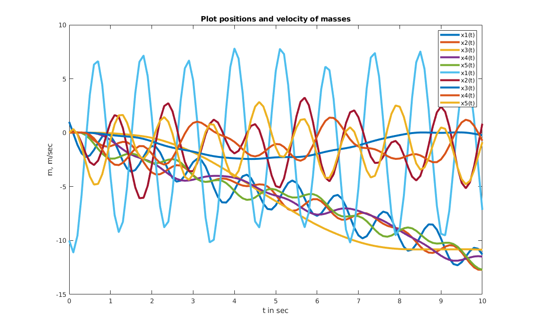
Note that the solution is not 100% correct, cause it was assumed, that all eigenvalues are single which they are not! For this reason actually another approach has to be used.

Stability

Bounded Input Bounded Output (BIBO) stability means that if you give e.g. a step on a system the output will not increase more and more but be limited.

A system is BIBO stable if:

• All eigenvalues \(\lambda_i\) are on the left half plane. If this is the case all eigen motion \(e^{\lambda_i t}\) will decrease.
• Hurwitz criteria
• Nyquist criteria for siso and mimo
• Bode Plot

PT1 and PT2

Matlab script (for the above plot)

%PT1 test:
%          K
%G(s) =  --------
%         1+sT
pt1 = tf(1,[0.1, 1])
step(pt1)
hold on;
pt11 = tf(1,[0.6, 1]);
step(pt11);
pt111 = tf(1,[0.2, 1]);
step(pt111);


%PT2 test:
%                  K
%G(s) =  ---------------------
%        T^2 s^2 + 2 D T s + 1
% T = 1/w_o (Time Constant)
% 0 < D < 1 Damping ratio
T = 0.6;
D = 0.5;
pt2 = tf(1,[T^2, 2*D*T, 1]);
o = exp((-pi*D/(sqrt(1-D*D))));
step(pt2);
T5pre = 3/abs(D*1/T)

% Notes Hold only for PT2
% For steady state (reach desired K value at t(end)) make sure that G(0) =1
%
%For overshoot:  o = e^(-pi*D / (sqrt(1-D^2)))  (circa)
% Within 5% band: T = 3/(abs(D*1/T))  (circa for D <0.8)

% Now let's say we want just o<=5% and T<1s
% --> -ln(o) /( sqrt(pi^2 + ln^2(o) ) = D
% --> T with try and error 1/T = 4.3 --> 
o = 0.05;
D = -log(o) / (sqrt(pi*pi + log(o)*log(o)))
T = 1/4.3
pt22 = tf(1,[T^2, 2*D*T, 1]);
step(pt22);

o = 0.1
D = -log(o) / (sqrt(pi*pi + log(o)*log(o)))
T = 1/7
pt23 = tf(1,[T^2, 2*D*T, 1]);
step(pt23)

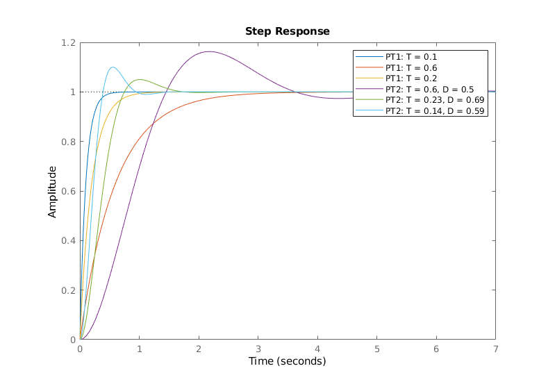
legend('PT1: T = 0.1 ', 'PT1: T = 0.6', 'PT1: T = 0.2', 'PT2: T = 0.6, D = 0.5', 'PT2: T = 0.23, D = 0.69', 'PT2: T = 0.14, D = 0.59');

Step Response

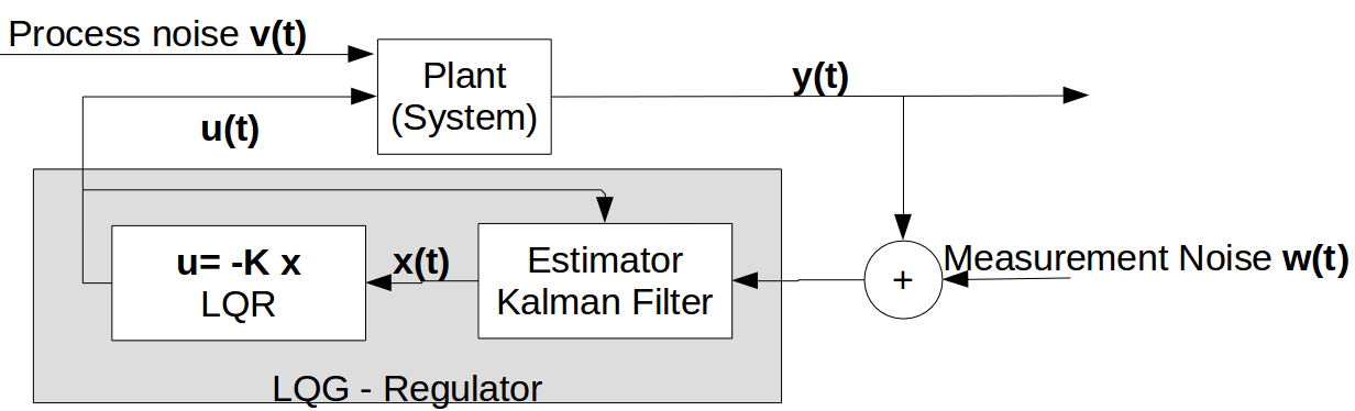
Control Circuit